Sag Calculation: Segment Equilibrium Method

Intro

In the previous article of this series, Sag Calculation: Parabola vs. Hyperbolic, I compared two classical analytical models and showed where the shallow sag assumption (\(dx \approx dL\)) breaks down. Both curves are closed-form and convenient. Both also assume a smooth wire under a continuous load.

A real span of an overhead contact system (OCS) or a power line rarely looks like that. In practice we deal with:

• concentrated loads along the span: droppers, clamps, insulators, bird diverters, ice sleeves;
• inclined spans with supports at different heights (\(y_A \neq y_B\));
• uneven weight distribution when the sag is deep and the wire slope changes sharply between the support and mid-span.

Stitching a separate cosh curve between every pair of droppers quickly becomes unmanageable by hand. A simpler engineering route is to split the wire into a finite number of straight segments and check static equilibrium one segment at a time.

This article covers the piecewise-linear sag approximation, also known as the Segment Equilibrium or Local Displacement Method. I run it in standard Excel 365 in three successive approximations, including elastic elongation, with dynamic array formulas (SEQUENCE, MAP, LAMBDA) and no VBA.

1. The Physical Model: From a Continuous Curve to Hinged Segments

Divide a span of horizontal length \({L}\) into \({N}\) straight rigid elements connected by frictionless hinges (nodes \(i = 0, 1, 2, \dots, N\)).

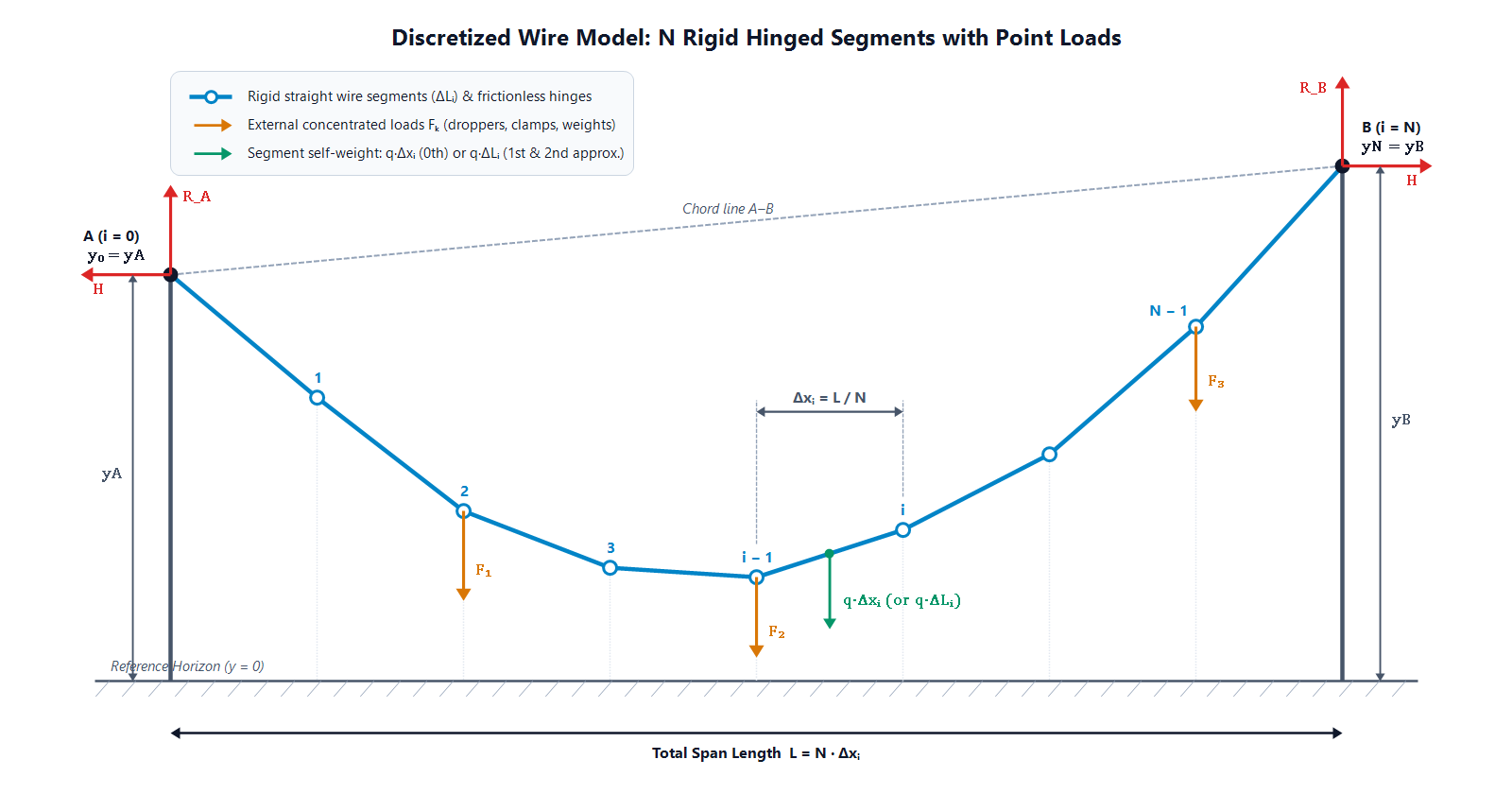
Discretized wire model: N rigid straight segments connected by frictionless hinges under self-weight and concentrated loads

The model rests on four assumptions:

• Equal horizontal steps. Every segment has the same horizontal projection \(\Delta x_i = L/N\).
• Zero bending stiffness. The nodes are ideal hinges with zero bending moment. For a flexible stranded conductor this is close to reality.
• Constant horizontal tension. As shown in the first article of the series, State Equation of a Freely Suspended Wire, without horizontal external loads the horizontal component \({H}\) is the same in every segment.
• Combined vertical load. Each segment \({i}\) carries its own weight (projected, \(q \cdot \Delta x_i\), or along the true length, \(q \cdot \Delta L_i\)) plus any concentrated vertical force \(F_i\) at that location.

2. Step-by-Step Equilibrium: No Matrices, No Iterations

With \({H}\) known, there is no stiffness matrix to invert and no solver to run. We march from the left support \(A(0, y_A)\) to the right support \(B(L, y_B)\).

Step 1: Support Reactions Ra and Rb

Taking moments of all vertical loads about support \({B}\), and then about support \({A}\), with the height difference of the supports included, gives the vertical reactions:

$$R_a = \frac{1}{L}\left[\sum_k F_k (L-x_k) + W_{wire}\frac{L}{2} - H(y_B-y_A)\right]$$

$$R_b = \frac{1}{L}\left[\sum_k F_k x_k + W_{wire}\frac{L}{2} + H(y_B-y_A)\right]$$

Check:

$$R_a + R_b = \sum_k F_k + W_{wire}$$

where

• \({L}\): horizontal span length, m;
• \(y_A\), \(y_B\): heights of the left and right supports, m;
• \({H}\): horizontal component of tension, N;
• \(F_k\): concentrated vertical load \({k}\) at horizontal distance \(x_k\), N;
• \(W_{wire}\): total self-weight of the wire in the span, N.

Remember the \(W_{wire} \cdot L/2\) term. It assumes the wire's center of gravity is at mid-span, and Section 5 shows what that costs.

Step 2: Equilibrium of the i-th Segment

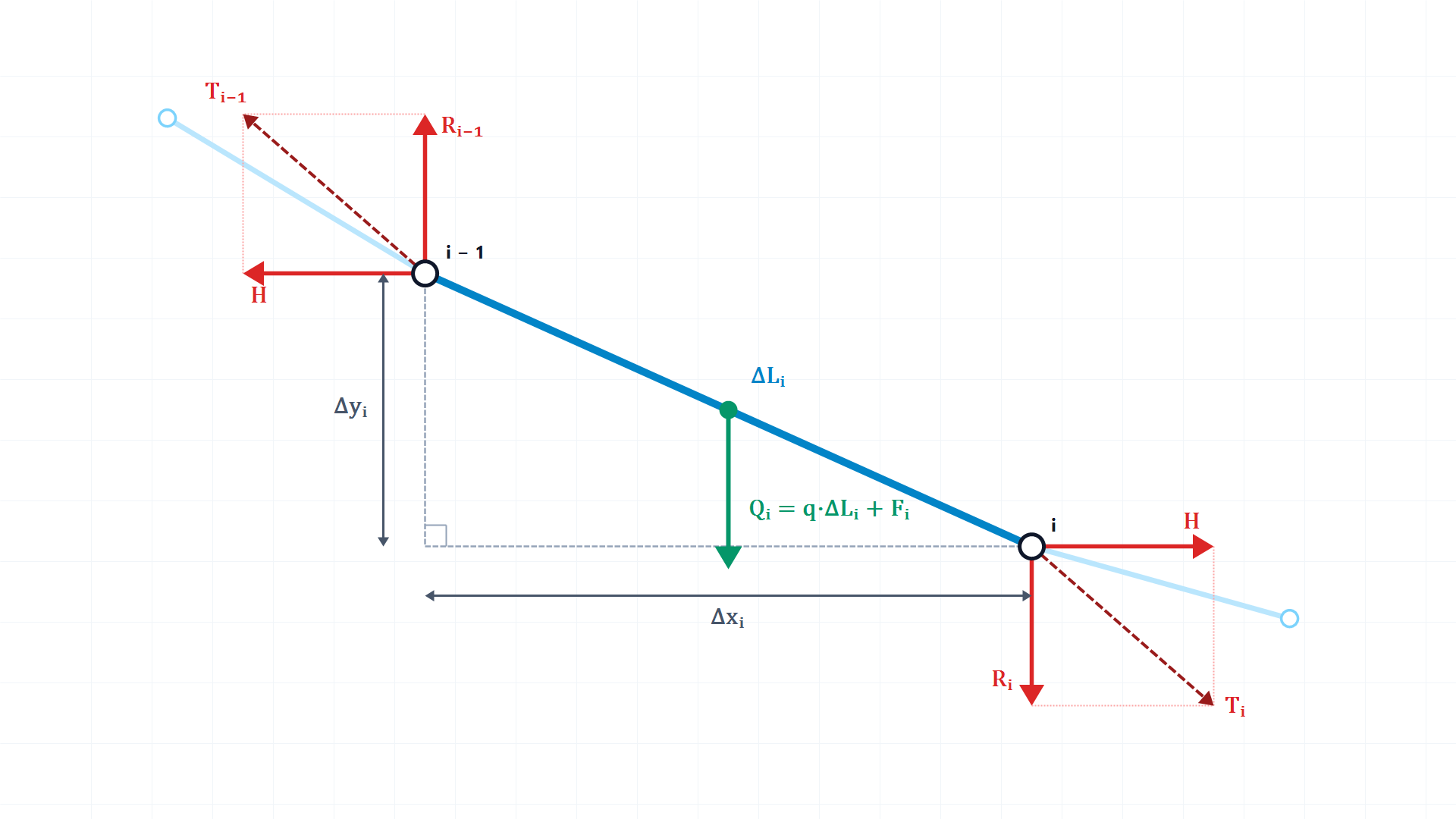
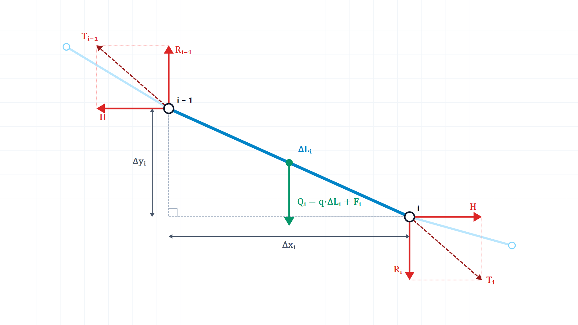
Now isolate the \({i}\)-th segment between nodes \(\mathit{(i-1)}\) and \({i}\).

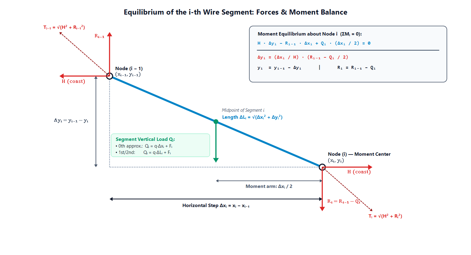
Free-body diagram of the i-th wire segment and moment balance about node i

At the left hinge (\(\mathit{i-1}\)), the rest of the wire pulls the segment with the horizontal force \({H}\) and the upward vertical force \(R_{\mathit{(i-1)}}\). The segment itself carries the total downward load \(Q_i\): its own weight plus any point load \(F_i\).

From node (\(\mathit{i-1}\)) to node \({i}\) the vertical internal force drops by \(Q_i\). To get the vertical drop \(\Delta y_i\), write the moment balance about the right hinge \({i}\), with \(Q_i\) applied at the segment midpoint (arm \(\Delta x_i / 2\)).

Vertical force balance:

$$R_i = R_{\mathit{(i-1)}} - Q_i$$

Moment balance about node \({i}\):

$$\sum M_i = 0: \quad H \Delta y_i - R_{\mathit{(i-1)}} \Delta x_i + Q_i \frac{\Delta x_i}{2} = 0$$

Vertical drop and node elevation:

$$\Delta y_i = \frac{\Delta x_i}{H}\left(R_{\mathit{(i-1)}} - \frac{Q_i}{2}\right), \qquad y_i = y_{\mathit{(i-1)}} - \Delta y_i$$

True length of the segment:

$$\Delta L_i = \sqrt{\Delta x_i^2 + \Delta y_i^2}$$

where

• \({i}\): segment and right-node index, from 1 to \({N}\); \(y_0 = y_A\), \(R_0 = R_a\);
• \(\Delta x_i\): horizontal step \(L/N\), m;
• \(\Delta y_i\): vertical drop across segment \({i}\), m;
• \(Q_i\): total vertical load on segment \({i}\) (self-weight plus \(F_i\)), N;
• \(R_i\): vertical component of wire tension at node \({i}\), N;
• \(\Delta L_i\): inclined length of segment \({i}\), m.

The algorithm is recursive. Starting from the left boundary (\(y_0 = y_A\), \(R_0 = R_a\)), each \(y_i\) comes directly from the previous node, so there is no simultaneous system to solve.

3. Three Successive Approximations and Elastic Elongation

In the previous article, the difference between the parabola and the hyperbolic cosine came down to one question: is the wire weight distributed along the horizontal projection (\({dx}\)) or along the true arc length (\({dL}\))?

The segment method covers both cases with successive approximations:

• 0th approximation, projected weight. The segment slopes are unknown at the start, so each segment weighs \(q \cdot \Delta x_i\): \(Q_i^{(0)} = q \cdot \Delta x_i + F_i\). One pass gives the drops \(\Delta y_i^{(0)}\) and lengths \(\Delta L_i^{(0)}\).
• 1st approximation, true length weight. With the inclined lengths known, the segment weight becomes \(Q_i^{(1)} = q \cdot \Delta L_i^{(0)} + F_i\). Steep segments near the supports are longer than \(\Delta x_i\), so they are heavier. The same formulas give new \(y_i^{(1)}\) and \(\Delta L_i^{(1)}\).
• 2nd approximation, refined weight. One more pass with \(Q_i^{(2)} = q \cdot \Delta L_i^{(1)} + F_i\) fixes the final geometry \(y_i^{(2)}\) and the strained wire length \(L = \sum \Delta L_i^{(2)}\).

A quick check for readers: set all point loads to zero (\(F_k = 0\)) in the workbook. The 0th approximation then reproduces the analytical parabola, and the 1st and 2nd approximations converge toward the cosh curve.

Elastic Elongation and Unstressed Length L₀

Once the geometry is final, both tension components are known in every segment: the constant \({H}\) and the local vertical \(R_i\). The axial tension \(T_i\) and the unstressed (manufactured) length \(\Delta L_{0,i}\) of each segment follow from Hooke's law:

$$T_{i} = \sqrt{H^{2} + R_{i}^{2}}, \qquad \varepsilon_{i} = \frac{T_{i}}{E A}$$

$$\Delta L_{0,i} = \frac{\Delta L_{i}}{1 + \varepsilon_{i}}, \qquad L_{0} = \sum_{i=1}^{N} \Delta L_{0,i}$$

where

• \(T_i\): axial tension in segment \({i}\), N;
• \(\varepsilon_i\): elastic strain of segment \({i}\);
• \({E}\): equivalent Young's modulus of the conductor, N/mm²;
• \({A}\): cross-sectional area of the conductor, mm²;
• \(\Delta L_{0,i}\): unstressed length of segment \({i}\), m;
• \(L_0\): total unstressed length of the wire in the span, m.

4. Stress-Testing the Model in Excel

To make the difference between the approximations visible, I pushed the model into a deep-sag, strongly asymmetric case on the "SEM" sheet of my workbook.

Input Data (Sheet "SEM")

Parameter	Value
Conductor	243-AL1 (EN 50182)
Cross-section \({A}\)	242.5 mm²
Young's modulus \({E}\)	55,000 N/mm²
Unit weight \({q}\)	6.5835 N/m
Span \({L}\)	40 m, \({N}\) = 40 segments, \(\Delta x_i\) = 1.0 m
Support heights	\(y_A\) = 10.0 m (left), \(y_B\) = 15.0 m (right)
Horizontal tension \({H}\)	100 N (deliberately low to get a deep sag)

Point loads (table addForce):

Load	\(F_k\), N	\(x_k\), m
\(F_1\)	50	10
\(F_2\)	10	20
\(F_3\)	0	30
\(F_4\)	30	35

Excel Implementation Without Macros

The algorithm is purely sequential, so it needs neither VBA loops nor Solver. In Excel 365 the whole 40-segment calculation spills from dynamic array formulas built on SEQUENCE, FILTER, MAP and LAMBDA. Three examples.

Node coordinates \(x_i\):

=SEQUENCE(N, 1, L/N, L/N)

Point loads \(F_i\) mapped to the nodes:

=MAP(S5#, LAMBDA(x, SUM(FILTER(addForce[F, N], addForce[x, m]=x, 0))))

Cumulative vertical force \(R_i\):

=Ra - MAP(SEQUENCE(ROWS(U5#)), LAMBDA(i, SUM(INDEX(U5#, 1):INDEX(U5#, i))))

Results of the Three Approximations

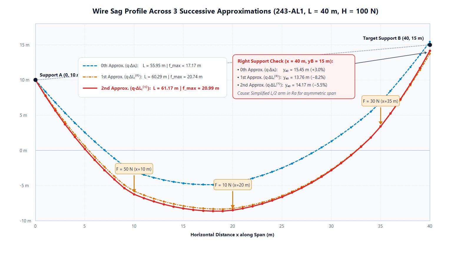
Comparison of the 0th, 1st and 2nd approximations for a 40 m inclined span with four point loads and H = 100 N

Parameter	0th approx. \(q \cdot \Delta x_i\)	1st approx. \(q \cdot \Delta L_i^{(0)}\)	2nd approx. \(q \cdot \Delta L_i^{(1)}\)
Total wire weight \(W_{wire}\), N	263.34	368.37	396.93
Left reaction \(R_a\), N	165.42	217.93	232.21
Right reaction \(R_b\), N	187.92	240.43	254.71
Strained wire length \({L}\), m	55.9532	60.2914	61.1744
Unstressed wire length \(L_0\), m			61.1736
Maximum sag \(f_{max}\), m	17.17	20.74	20.99
Computed right end \(y_{40}\), m	15.45	13.76	14.17
Right support error vs. \(y_B\)	+3.00%	−8.26%	−5.53%

The gap between the 0th approximation (\(f_{max}\) = 17.17 m, \({L}\) = 55.95 m) and the 1st and 2nd (\(f_{max}\) = 20.99 m, \({L}\) = 61.17 m) is large. At \({H}\) = 100 N, distributing the weight over the horizontal projection (\(q \cdot \Delta x_i\)) underestimates the wire weight in the span by more than 33% (263.3 N vs. 396.9 N).

The method settles fast: between the 1st and 2nd approximations the maximum sag changes by only 0.25 m (20.74 m vs. 20.99 m).

5. Why the Curve Misses the Right Support

The last two rows of the table (rows 44 and 45 on the "SEM" sheet) show a problem. The march starts at \(y_0 = y_A\) = 10.00 m, crosses \({N}\) = 40 segments and reaches \({x}\) = 40 m. The last node \(y_{40}\) should land on the right support, \(y_B\) = 15.00 m. It does not:

• 0th approximation: \(y_{40}\) = 15.45 m (+0.45 m, +3.0%);
• 1st approximation: \(y_{40}\) = 13.76 m (−1.24 m, −8.3%);
• 2nd approximation: \(y_{40}\) = 14.17 m (−0.83 m, −5.5%).

This is not an error in the workbook. Two simplifications in the textbook form of the method produce exactly these offsets.

The +0.45 m Offset in the 0th Approximation: Midpoint vs. Node

In the reaction \(R_a\), the point loads \(F_k\) act at the nodes \({x}\) = 10, 20 and 35 m) with their exact arms \(L-x_k\). In the segment equation for \(\Delta y_i\), the same \(F_i\) is part of \(Q_i = q \cdot \Delta x_i + F_i\) and is halved. This moves it from the hinge \(x_i\) to the segment midpoint \(x_i-\Delta x_i/2\). Over the span the half-step shift adds up to:

$$\Delta y_{offset} = \frac{\Delta x \cdot \sum_{k} F_{k}}{2H}$$

With \(\Delta x\) = 1.0 m, \({H}\) = 100 N and loads of 50, 10 and 30 N:

$$\Delta y_{offset} = \frac{1.0}{2 \cdot 100}(50 + 10 + 30) = 0.45~\mathrm{m}$$

The −0.83 m Offset in the 1st and 2nd Approximations: Center of Gravity

The 1st and 2nd approximations still use \(W_{wire} \cdot L/2\) in the reactions, so the wire's center of gravity stays at mid-span (\(L/2\) = 20 m). For a uniform load \(q \cdot \Delta x_i\) this is exact. With true segment lengths \(q \cdot \Delta L_i\) in an inclined, unevenly loaded span, the segments on the steeper side are longer and therefore heavier, and the center of gravity moves away from \(L/2\). Keeping \(L/2\) in \(R_a\) underestimates the starting reaction, and the curve ends below \(y_B\) = 15.00 m.

6. Conclusions

1. At working tensions the boundary error is negligible. \({H}\) = 100 N is an extreme case: the sag exceeds half the span, which magnifies every nonlinear effect. With a realistic \({H}\) = 10,000 N (10 kN) on the "SEM" sheet, the right support error drops below 0.03% (about 4 mm), and the three approximations practically coincide.
2. Where the method fits:
   • spans with point loads (droppers, insulators, weights), inclined supports and a known horizontal tension \({H}\);
   • a fast, transparent spreadsheet model with no iterations, VBA or FEM software;
   • an independent check of complex spans.

The workbook is free to download: Excel file, sheet "SEM". Two experiments worth trying on the "SEM" sheet:

• raise \({H}\) from 100 N to 5,000 N and watch the three approximations and the right support error converge;
• set all point loads in the addForce table (D3:D6) to 0 and compare the 0th and 2nd approximations with the parabola and cosh calculator from the previous article.

Limits and the Next Step

The method handles uneven loading well, but it has two limits. It needs the horizontal tension \({H}\) in advance, and its simplified reaction formula drifts at the right support when the sag is deep and asymmetric.

In real design \({H}\) is often the unknown, while the unstressed wire length \(L_0\) is fixed. The next article in the series moves to the iterative nodal (tangent) method, which solves for exact equilibrium at every node for a given unstressed length.